When a language model processes text, it must determine how much the context of one token helps explain the meaning of another. This depends on both content (a dog should attend more strongly to puppy than tshirt) and relative position - the word cat appearing in the same sentence has far more semantic influence than the same word, cat, appearing chapters away. Without positional information, Transformers are permutation-invariant and cannot distinguish between these cases.

Rotary Position Embeddings (RoPE) elegantly solve this by rotating query and key vectors based on their positions before computing attention scores¹. Rather than adding positional embeddings to tokens, RoPE bakes position-awareness directly into the query-key interactions. This approach naturally captures relative positions, extends to arbitrary sequence lengths, and allows different attention heads to learn different position-sensitivity patterns.

This post examines RoPE from first principles. We’ll start with a review of traditional positional embeddings and their limitations, then derive RoPE’s mathematical formulation from 2D rotations to the general case. We’ll explore why it works so well in practice, and finish with implementation details and real-world performance considerations.

Attention Recap

Attention scores are computed as follows.

Let’s consider the input vectors $\mathbf x_m$and $\mathbf x_n$ at positions $m$ and $n$ respectively. In the first layer, these vectors are the initial token embeddings. In any subsequent layer, they are the hidden states output by the previous layer. To calculate the attention score that is the interest $\mathbf x_m$ has in $\mathbf x_n$ we compute:

Query: $\mathbf q_m = \mathbf W_q\mathbf x_m$

Key: $\mathbf k_n= \mathbf W_k\mathbf x_n$

Where $\mathbf W_q$ and $\mathbf W_k$ are projection matrices for creating queries and keys respectively. The query is a vector that encodes a description of the other inputs that position $m$ is interested in. The key is a vector that encodes a description of the input at position $n$. The model learns weights $\mathbf W_q$ and $\mathbf W_k$ such that this is true.

When, $\mathbf q_m$ and $\mathbf k_n$ are similar, $\mathbf x_n$ matches the description of tokens $\mathbf x_m$ is interested in. Therefore, we construct the attention score as a measure of this similarity - the dot product!

$\mathbf A_{m,n}=\mathbf q_m^\top \mathbf k_n$

Different attention heads have different query and key projections such that the descriptions differ in content allowing them to search for different types of content.

In this construction, the attention score depends only on the content of the embeddings $\mathbf x_m$ and $\mathbf x_n$. Therefore, the classic approach for positional encoding is to add a positional encoding vector to these embeddings.

Absolute Positional Embeddings

The traditional approach to positional embeddings is to create an embedding vector $\mathbf p_m$ dependent only on the absolute position $m$ and add that to the token embedding $\mathbf x_m$ before the first layer of the transformer:

$\mathbf e_m=\mathbf x_m+ \mathbf p_m$

where $\mathbf{e}_m$ is the final embedding combining token and position information.

The skip connections in the transformer architecture and the fact that the embedding is added mean that the positional embedding is a component of the input at all the layers and doesn’t have to be reintroduced.

Learnt Embeddings

The simplest way to implement positional embeddings is to get the model to learn them. This can be implemented as a large embedding table with an entry for each position.

In modelling language, typically it is the relative positions of tokens to one another which matter, not their absolute positions. When learning embeddings from scratch like this the model has no prior on the relationships between positions - it doesn’t even know that 4 comes after 3. Therefore, it has the hard task of learning to embed positions in a way that the attention score is (somewhat) dependent on the relative positions of the two inputs.

Moreover, these embeddings are strictly limited to the context length seen during training since each position must have its own entry in the table.

This approach therefore trades any kind of built-in positional understanding for complete flexibility. However, it’s not clear this flexibility offers a real-world performance advantage over a well-designed, engineered method. For these reasons, especially the hard limit on sequence length, many modern architectures have moved towards alternative approaches.

Sinusoidal Embeddings

A different approach, introduced in Attention Is All You Need², is to fix the positional embeddings to be a sinusoidal function on the position defined as:

The original paper suggests that this embedding might “allow the model to easily learn to attend by relative positions, since for any fixed offset $j$, $\mathbf p_{m+j}$ can be represented as a linear function of $\mathbf p_m$”². Further analysis in Transformer-XL³ identifies the position-position term in the attention score: $\mathbf p_m^\top \mathbf W_q^\top \mathbf W_k \mathbf p_n$, as being responsible for the relative positional effects on the score. Therefore, the model has to learn $\mathbf W_q$ and $\mathbf W_k$ such that this term as well as the other 3 terms (content-content, content-position, position-content) each have the intended effect on the attention score.

Even if we don’t fully understand how these positional embeddings interact in the attention mechanism due to the projection matrices, the validity of this engineered approach is reinforced by a fascinating discovery.

Subsequent research has shown that models using purely learned embeddings actually learn sinusoid-like patterns on their own⁴. This discovery could explain why the original “Attention Is All You Need” paper found that both methods performed roughly equally—the learned approach may simply be rediscovering the effective, frequency-based patterns of the sinusoidal one. Ultimately, this suggests that the sinusoidal pattern may be a core component of the optimal approach for modeling sequences in Transformers.

RoPE Formulation

In deriving RoPE, the authors wanted to take a more direct approach with a more predictable effect on the attention scores. They started by defining the final query and key vectors, $\mathbf q_m$ and $\mathbf k_n$, as functions that depend on both the content $\mathbf{x}$ and the position $m$:

The goal is to find functions $f_q$ and $f_k$ such that there exists a function $g$ that depends only on the content and the relative distance $m-n$.

Further, these functions, $f_q$ and $f_k$, must also perform the standard learned projections ($\mathbf W_q$ and $\mathbf W_k$). Therefore, the problem includes a base case: at an abstract position 0 where no positional information is applied, the functions should simply return the normal projection of the input vector:

RoPE Solution

To understand their solution, first recall that the dot product of two vectors is a measure of their angular alignment scaled by their magnitudes. Therefore, rotating one vector away from the other will decrease their dot product. This gives us a mechanism to encode distance $m-n$: the further apart two inputs are, the more we rotate the key away from the query. The challenge is to create this effect using only information about absolute positions.

The key insight is that rotating $\mathbf{q}$ by $m\theta$ and $\mathbf{k}$ by $n\theta$ is geometrically equivalent to first rotating $\mathbf{q}$ by $(m-n)\theta$ and then rotating both resulting vectors by $n\theta$. Since rotating both vectors by the same amount doesn’t change their dot product, the final dot product is the same as the one between $\mathbf{q}$ rotated by $(m-n)\theta$ and the original vector $\mathbf{k}$.

Therefore, we have the property:

where, in the 2-d case, $\mathbf R_m$ is the 2-d rotation matrix:

This gives the solution:

This property allows us to use rotations based on absolute positions to affect attention scores in a way that is dependent only on the relative positions.

n-D Case

So far we’ve just shown the case where the embedding dimension is 2. Expanding this to the n-dimensional case is surprisingly simple. We treat each pair of dimensions as a 2D subspace and apply the rotation there, leaving other dimensions unchanged. This results in a block-diagonal matrix:

Because each pair of dimensions is treated independently, this generalisation also satisfies the conditions set out above.

Now is a good time to discuss the values of $\theta$. Because $\sin$ and $\cos$ are periodic functions, the positional encoding of each pair of dimensions—or “channel”—is also periodic with a frequency determined by $\theta_i$. The designers of RoPE chose to use the geometric function:

The aggregate effect of combining these different frequencies is that attention scores naturally decay with relative distance, a property that aligns well with the decay of relevance in natural language. More strictly, the authors find an upper bound on the attention score which can be decomposed into a content-dependent part and a position-dependent part. Plotting the position-dependent part of this upper bound (”relative upper bound”) shows this decay:

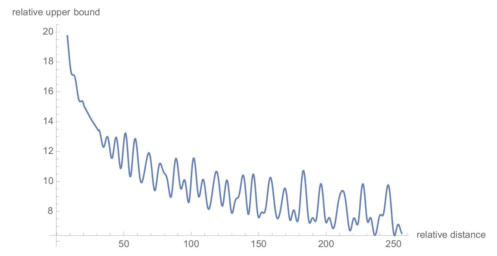Figure from Su, et al. (2021)¹

While this doesn’t guarantee that the attention score for a specific query and key will strictly decrease with distance, the analysis proves that the maximum possible score gets smaller. This acts as a shrinking ceiling, creating a strong bias that naturally dampens attention between distant tokens.

Varying the decay

Crucially, the exact decay profile for any two tokens is content-dependent. This is not merely a caveat; different types of relationships require different decay shapes. For instance, the token “cat” should only attend to a directly preceding “a” or “the”, requiring a very sharp decay. Meanwhile, it may need to attend to instances of “kitten” much further away to get relevant context, which requires a gentle decay.

The model learns to achieve this by using the projection matrices ($\mathbf W_q$ and $\mathbf W_k$) to route information. For sharp, local dependencies, it learns to place information into the high-frequency channels (early dimensions). For gentle, long-range dependencies, it places information into the low-frequency channels (late dimensions).

Therefore, the base (10,000) is a key architectural choice when using RoPE since this controls the range of frequencies available, and thus how sharp or shallow the decays can be.

Base

Because the individual embedding dimensions are periodic, the choice of base also puts a soft limit on the maximum sequence length RoPE can meaningfully be used for. Beyond this limit, the model can struggle to distinguish the relative positions of tokens.

A key advantage of RoPE, however, is that its mathematical structure allows this limitation to be addressed in a principled way. By adjusting the rotational frequencies at inference time, researchers have enabled models to work with context lengths much longer than they were trained on⁵. Amongst other algorithmic improvements, this made RoPE a key part in enabling test-time compute. For those interested in the technical details, a popular family of techniques for this is known as NTK-scaling.

Training Dynamics and Model Quality

We’ve now seen the mathematical elegance of RoPE as a positional embedding and argued for its advantageous theoretical properties, but how does it affect training performance? The original paper demonstrates a clear advantage in training efficiency. Their experiments show a BERT-style model using RoPE converges significantly faster and reaches a lower final loss than a standard BERT with learned position embeddings. This faster convergence likely stems from RoPE’s built-in decay characteristic. The model can immediately attend to nearby tokens without first having to learn that proximity matters. This allows it to focus on learning semantic relationships from the very start.

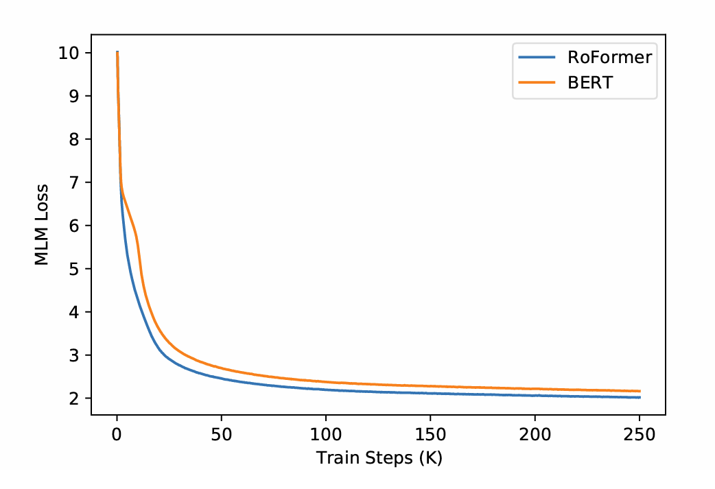Figure from Su, et al. (2021)¹

Moreover, the authors also demonstrate a distinct advantage on longer sequence lengths. On a long-document matching task, RoFormer’s advantage over the baseline grew even larger when the context was extended to 1024 tokens—a significant achievement at a time when the 512-token context length was a standard limitation for most models.

This early advantage has been proven effective at scale. It’s a key reason why RoPE continues to be the go-to positional embedding for today’s open-source SOTA models, including Deepseek V3 (with a 128k token context window)⁶ and Llama 4 (with a context window of over 1 million tokens)⁷.

Implementation

For complete implementations see my repo.

The rotation matrices are sparse meaning that implementing them as is requires an inefficient large matrix multiplication. The authors offer a more efficient approach which involves only the necessary multiplications¹.

Note: $\odot$ refers to the element-wise (Hadamard) product. The paper incorrectly uses $\otimes$ which conventionally refers to the tensor (Kronecker) product, causing some confusion.

This formula is gnarly to express directly in terms of $m$, $\Theta$ and $\mathbf x$ due to the mixing of indices in each pair as well as the half speed counting of index $i$ on $\theta$. To simplify this, we can reshape the vectors into matrices with two columns, which means the rows are now indexed directly with $i$.

This gives:

This indexing provides a more elegant implementation:

# Reshape input into odd and even indices
x_paired = x.reshape(*x.shape[:-1], self.dim // 2, 2)
x_odd, x_even = x_paired[..., 0], x_paired[..., 1]

# Apply the rotation
x_out_odd = x_odd * cos - x_even * sin
x_out_even = x_odd * sin + x_even * cos

# Combine back and flatten
x_out = torch.stack([x_out_odd, x_out_even], dim=-1).flatten(3)

We can build the cos and sin tensors with:

freq_indices = torch.arange(0, self.dim, 2, dtype=self.dtype, device=self.device)
exponents = - freq_indices / self.dim
theta = self.base ** exponents # [dim // 2]

position_indices = torch.arange(self.max_seq_len, dtype=self.dtype, device=self.device)

# Outer product: [max_seq_len, 1] * [1, dim // 2] -> [max_seq_len, dim // 2]
angles = position_indices.unsqueeze(1) * theta.unsqueeze(0)
angles = angles.float() # ensure float32 for sin and cos accuracy

cos = torch.cos(angles)
sin = torch.sin(angles)

# Add a heads dimension for broadcasting
cos = cos.unsqueeze(-2) # [..., seq_len, 1, dim//2]
sin = sin.unsqueeze(-2) # [..., seq_len, 1, dim//2]

Choice of pairs (the half-flipped method)

As we see with this implementation, the interleaving of the two cases makes the implementation complex. However, the choice to pair up adjacent dimensions for the rotations is entirely arbitrary. The key property is preserved no matter how we pair them up. A particularly neat choice is to split the vectors into the first and second half and pair the dimensions of each half⁸: (1, d/2 + 1), (2, d/2 + 1) … (d/2, d).

Let $\mathbf x^*$ be the third vector in the formula. Explicitly:

This can be implemented as:

cos = torch.cat([cos, cos], dim=-1)
sin = torch.cat([sin, sin], dim=-1)

# Create the third vector
x_first_half, x_second_half = x.chunk(2, dim=-1)
x_half_flipped = torch.cat([-x_second_half, x_first_half], dim=-1)

# Apply the rotation
x_out = (x * cos) + (x_half_flipped * sin)

When benchmarking these two approaches, I found that the half-flipped method outperformed the interleaved method when uncompiled. However, when using torch.compile this advatage disappeared and the performance was almost identical.

Performance, Memory and Caching

Currently, the most expensive parts of this embedding are the creation of the sin and cos tensors, therefore we want to reuse these computations as much as possible. One option is to cache these values in a buffer when the RoPE module is created. This caching strategy, while essential for performance, introduces its own significant cost: a new and substantial memory footprint which must be carefully managed in modern LLM architectures. To illustrate this, let’s analyse the memory required by the RoPE cache for the Llama 3 70B architecture.

Llama 3 70B dimensions⁹:

• Head dimension: 128
• Number of layers: 80
• Context length: 128k (with RoPE scaling extension)
• Data type: bfloat16 (2 bytes)

This gives a total cache size of:

To put this into context we need to consider the other memory usage in the model: the weights and kv cache.

Llama 3 70B uses Grouped-Query attention with only 8 key-value heads⁹. Therefore the KV cache is:

Using bfloat16, the model weights take up:

This makes the RoPE cache seem insignificant. However, when using tensor parallelism, say across 8 GPUs, the weights and KV cache are split across the GPUs while the RoPE cache is duplicated. Per GPU, this gives:

• Weights: 16.3 GiB
• KV cache: 5 GiB
• RoPE cache: 5 GiB

And the RoPE cache is now significant.

The Factory Pattern

Recognising that the same embedding is created and applied at each layer during a forward pass provides another dimension for reuse. In the factory design pattern, we create an embedding once at the beginning of the model and pass it through the model to be applied at each layer. This removes the factor of number of layers from the cache calculation which in deep models is particularly significant.

Without this pattern, storing a separate cache in each of the 80 layers results in significant memory duplication. The key insight is that every layer uses the exact same positional embedding, so we can remove the duplication by creating it only once.

This is the principle behind the Factory Pattern. In this design, we create an embedding once at the beginning of the model and pass it through the model to be applied at each layer. This removes the factor of number of layers from the cache calculation. Specifically, the embedding created is the sin and cos tensors for the required positions.

Let’s update the analysis with the factory pattern, removing the factor of 80 layers:

The factory pattern also presents a final design choice: What exactly should be cached? To handle inference for any token, we have two options:

1. Pre-compute and cache the full sin/cos table for the entire context window (e.g., 64 MiB for 128k context). This makes fetching embeddings a fast memory lookup.
2. Cache only the tiny theta tensor (the rotation frequencies) and compute the sin/cos values on the fly as needed.

During autoregressive generation, we only need the embeddings for a single new token at each decoding step because the kv cache already has the positions embedded. In this case, the second approach is vastly more memory-efficient.

Conclusion

Since its introduction in 2021, RoPE has quickly become the de facto standard for positional encoding in modern LLMs. The method achieves relative position-dependent attention scores without explicitly encoding every possible pair of positions, and integrates seamlessly with KV caching since positional information is baked directly into the cached keys and values. The attention scores exhibit a natural decay with relative distance, aligning well with how relevance diminishes over distance in natural language, and the model can learn to control this decay rate by routing information through different frequency channels. Combined with its parameter-free nature and efficient implementation, RoPE has become the default choice in virtually every major open-source language model⁶⁹¹⁰.

References